BitNet: Scaling 1-bit Transformers for Large Language Models review and derivation

This article is review and derivation of Wang et al., BitNet: Scaling 1-bit Transformers for Large Language Models. 2023

Introduction

• I don’t think there’s anything unique about human intelligence. All the neuron is the brain that make up perceptron and emotion operate in binary fashion – William Henry Gates III

• The rapid growth of large language models has led to significant improvements in various tasks
  • However, it is expensive to host large language models due to the high inference costs and energy consumption
  • As the size of these models grows, the memory bandwidth required for accessing and processing the model parameters becomes a major bottleneck
• Model quantization has emerged as a promising solution, as it can significantly reduce the memory footprint and computational cost while maintaining competitive performance
  • Most existing quantization approaches for large language models are post-training
    • They are simple and easy but will result in a more significant loss of accuracy because the model is not optimized for the quantized representation during training
• Another strand of quantizing deep neural networks is quantization-aware training
  • It typically results in better accuracy, as the model is trained to account for the reduced precision from the beginning
  • The model becomes more difficult to converge as the precision goes lower
  • It is unknown whether quantization-aware training follows the scaling law of neural language models

• In this work, the authors focus on binarization, which is the extreme case of quantization, applied to large language models

• Previous studies on binarized neural networks have mostly revolved around convolutional neural networks

• Recently, there has been some research on binarized transformers
  • However, these studies have focused on machine translation or Bidirectional Encoder Representation from Transformers(BERT)
  • Machine translation employs an encoder-decoder architecture and BERT pretraining utilizes a bidirectional encoder, while large language models use a unidirectional decoder
• The authors propose BitNet, a 1-bit transformer architecture for large language models, which aims to scale efficiency in terms of both memory and computation
  • The implementation of the BitNet architecture require only the replacement of linear projections like nn.Linear in PyTorch

BitNet

• BitNet uses the same layout as transformers, stacking blocks of self-attention and feed-forward networks
  • BitNet uses BitLinear instead of conventional matrix multiplication, which employs binarized model weights
• Leave the other components high-precision, e.g., 8-bit
  • The residual connections and the layer normalization contribute negligible computation costs to large language models
  • The authors preserve the precision for the input/output embedding because models have to use high precision probabilities

    BitLinear

• Binarize the weights $\mathbf{W} \in \mathbb{R}^{n \times m}$ to either -1 or 1 with the signum function, where n is input dimension and m is output dimension
• The weights are centralized to be zero-mean before binarization to increase the capacity within a limited numerical range

\[\tilde{\mathbf{W}} = Sign(\mathbf{W} - \alpha),\] \[\text{ where } Sign(\mathbf{W}_{ij}) = \begin{cases} +1, \text{ if } \mathbf{W}_{ij} > 0 \\ -1, \text{ if } \mathbf{W}_{ij} \leq 0 \end{cases} \text{ and } \alpha = \frac{1}{nm}\sum_{ij}\mathbf{W}_{ij}\]

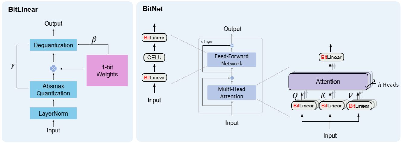
(Figure 1. (a) The computation flow of BitLinear. (b) The architecture of BitNet, consisting of the stacks of attention and Feed Forward Networks(FFNs), where matrix multiplication is implemented as BitLinear)

absmax quantization

• Before 1-bit weights multiplication, the activations are quantized to $b$-bit precision

• BitNet uses absmax quantization, which scales activation into the range $[-Q_b, Q_b], \text{ where } Q_b = 2^{b-1}$ by multiplying with $Q_b$ and dividing by the absolute maximum of the input matrix \(\tilde{x} = Quant(x) = Clip(x \times \frac{Q_b}{\gamma} - Q_b + \epsilon, Q_b - \epsilon) \\ Clip(x, a, b) = \max(a, \min(b, x)), \gamma = \|x\|_{\infty}\)

• Where 𝜖 is a small floating-point number that prevents overflow when performing the clipping

• For the activations before the non-linear functions like Rectified Linear Unit(ReLU), they are scaled into the range $[0,𝑄_𝑏]$ by subtracting the minimum of the inputs

\[\tilde{x} = Quant(x) = Clip\left((x - \eta) \times \frac{Q_b}{\gamma}, \epsilon, Q_b - \epsilon\right), \eta = \min_{ij} x_{ij}\]

• The matrix multiplication can be written as $y=\tilde{\mathbf{W}}\tilde{x}$

Dequantization

• A scaling factor \(\beta=\frac{1}{nm}\|W\|_{1}\approx \sigma_W=\frac{1}{\sqrt{n}}\) ,is used after binarization to reduce the l2 error between the real-valued and the binarized weights, \(\tilde{w_\beta}=\beta \cdot \tilde{w}\)

• $W$ is initialized with Kaiming (or Xavier method), which initialize weight $N(0,\frac{1}{\sqrt{n}})$

• Elements in $\mathbf{W} \in \mathbb{R}^{n \times m}$ and $x$ are mutually independent and share the same distribution, the variance of the output $y$ is \(\text{Var}(y)=n\text{Var}(\tilde{w_\beta}\tilde{x})=n \textbf{E}[\tilde{w_\beta}^2]\textbf{E}[\tilde{x}^2]=n\beta^2 \textbf{E}[\tilde{x}^2] \approx \textbf{E}[\tilde{x}^2]\)

• $\because \text{Var}(A)=\textbf{E}[A^2] - \textbf{E}[A]^2$, where $\textbf{E}[A]= \sum_x xp(x)$ (expectation value)
  • Average of $\tilde{w}$ is 0, because $\textbf{W}$ is initialized with random number with average=0
  • Average of $\tilde{x}$ is 0, because $\tilde{x}$ is layer-normalized
  • $\tilde{w}$ is -1 or 1, therefore $\textbf{E}[\tilde{w}^2]=1$
  • With scaling parameter $\beta$, $\textbf{E}[\tilde{w_\beta}^2]=\beta$
• Derivation of $\frac{1}{nm} |\textbf{W}|_1 \approx \frac{1}{\sqrt{n}}$
  • In a distribution with a mean of zero, the expected value of the absolute value can be approximated by the standard deviation, $\textbf{E}[|\textbf{W}|] \approx \frac{1}{\sqrt{n}}$
    • For more derivation details, please see Appendix
  • $\textbf{W}$ follow the law of large number because input size of$ Q,K,V$ matrix is 12288 in GPT-3
  • \[\therefore \frac{1}{nm} \|\textbf{W}\|_1 = \frac{1}{nm} \sum_{i=1}^{nm} |w_i|=\textbf{E}[|W|] \approx \frac{1}{\sqrt{n}}\]
• Role of $\beta$
  • With using standard initialization method, $\textbf{E}[\textbf{W}^2]=\frac{1}{n}$
    • For matching variance of y and variance of x because $\text{Var}(y)=n\text{Var}(wx)=n\text{Var}(w)\text{Var}(x)$
    • Standard initialization method initialize weights with $N(0,\frac{1}{n})$
  • Since square of both -1 and 1 is 1, $\textbf{E}[\tilde{w}^2]=1$
  • To maintain the variance of W after binarization, $\beta$ is important \(\because \textbf{E}[\tilde{w_\beta}^2]=\textbf{E}[\beta^2\tilde{w}^2]=\beta^2\textbf{E}[\tilde{w}^2]=\frac{1}{n}\)

  • Note that $ \beta=\frac{1}{nm}|W|_{1}\approx \sigma_W$ will be changed during training, however, $ \textbf{E}[\tilde{w}^2]$ is always 1. Therefore, to maintain the variance of W after binarization, $\beta$ is important since \(\because \textbf{E}[\tilde{w_\beta}^2]=\textbf{E}[\beta^2\tilde{w}^2]=\beta^2\textbf{E}[\tilde{w}^2]=\sigma_W^2\)

  • Since $\alpha$ is subtracted from original $W$, $E[\tilde w]=0$

Layer Normalization

• For the full-precision computation, the variance of the output $\text{Var}(y)$ is at the scale of 1 with the standard initialization methods like Kaiming or Xavier initialization
  • These methods have a great benefit to the training stability
• To preserve the variance after quantization, LayerNorm(LN) function is used before the activation(x) quantization
  • $\text{Var}(y) \approx \textbf{E}[\tilde{x}^2]=1$
  • It has exact implementation as SubLayerNorm(SubLN)(Wang et al., 2022)
• The output activations are rescaled with (𝛽,𝛾)
  • 𝛽 for scaling weights, 𝛾 for dequantization \(y = \tilde{\textbf{W}}\bar{x} = \tilde{\textbf{W}} \, Quant(LN(x)) \times \frac{\beta\gamma}{Q_b} \\ LN(x) = \frac{x-E(x)}{\sqrt{Var(x)+\epsilon}}, \; \beta = \frac{1}{nm}\|\textbf{W}\|_1\)

Model parallelism

• Technique to scale up large language models is model parallelism, which partitions the matrix multiplication on multiple devices
• A prerequisite for the model parallelism approaches is that the tensors are independent along the partition dimension
• However, all of the parameters 𝛼,𝛽,𝛾, and 𝜂 are calculated from the whole tensors, breaking the independent prerequisite
• Synchronization is growing as the model becomes deeper

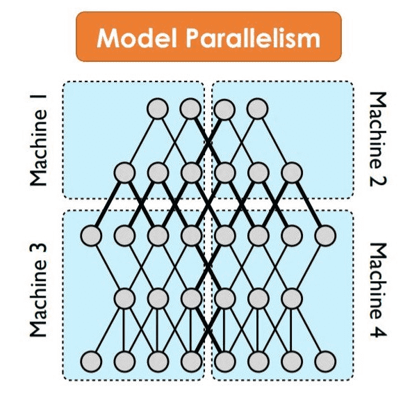
(Figure 2. Model parallelism)

• So, Divide the weights and activations into group and then independently estimate group’s parameters

• For weight matrix $\mathbf{W} \in \mathbb{R}^{n \times m}$, it is divided into G groups along the partition dimension(Each group has size of $\frac{n}{G} \times m$) \(\alpha _g = \frac{G}{nm}\sum_{ij}\mathbf{W}_{ij}^{(g)}, \beta _g=\frac{G}{nm}\|W^{(g)}\|_{1}\)
  • where $W^{(g)}$ is the g-th group of the weight matrix
• For input matrix $x \in \mathbb{R}^{n \times m}$, it is divided into G groups and calculate the parameters of each group \(\gamma _g = \|x^{(g)}\|_{\infty}, \eta _g= \min_{ij} x_{ij}^{(g)}\)
• For LN, compute the mean and variance for each group independently \(LN(x^{(g)}) = \frac{x^{(g)}-E(x^{(g)})}{\sqrt{Var(x^{(g)})+\epsilon}}\)

Model training

Straight-through estimator(Bengio et al., 2013)

• Employ the straight-through estimator to approximate the gradient during backpropagation
• Bypass the non-differentiable functions, such as Sign and Clip function
• Gradients flow through the network without being affected by non-differentiable function
• For stochastic binary neuron where the output $h$ is sampled as a binary value, the gradient of the loss $L$ with activation $a$ is simply $\frac{\partial L}{\partial a} = \frac{\partial L}{\partial h}$, where $a=f(h)$ with non-linear function $f$
  • Assume that the binary neuron function as identity function during backpropagation

(Figure 3. Sign function)

Mixed precision training

• While the weights and the activations are quantized to low precision, the gradients and the optimizer states are stored in high precision to ensure straining stability and accuracy
• Maintain a latent weight in a high-precision format for parameter updates
• Latent weights are binarized on the fly during the forward pass
  • This latent weights never used for the inference process

Large learning rate

• Small update on the latent weights often makes no difference in the 1-bit weights
  • This problem is even worse at the beginning of the training, where the models are supposed to converge as fast as possible
• Increasing learning rate is the simplest and best way to accelerate the optimization
• BitNet benefits from a large learning rate in terms of convergence, while the FP16 transformer diverges at the beginning of training with same learning rate

(Figure 4. Example of loss convergence during training)

Computational efficiency

Arithmetic operation energy

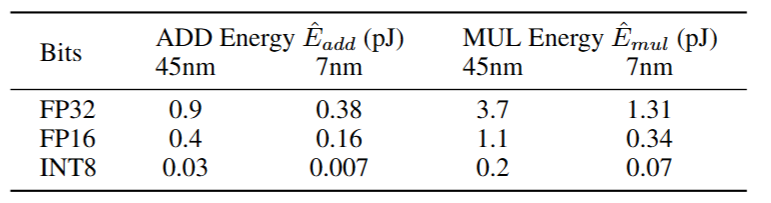
• The energy consumption for different arithmetic operation can be estimated as Table 2

• In vanilla transformers, for matrix multiplication with dimensions $ m\times n$ inputs and $n\times p$ weights, the number of addition is $m\times(n−1)×p$, and multiplication is $m\times n\times p$
• For BitNet, the multiplication are only applied to scale the output with the scaler $\beta$ and $\frac{\gamma}{Q_b}$, and absmax quantization for input, so the number of multiplication is $m\times p+ m\times n$
• BitNet provides significant energy saving, especially for the multiplication

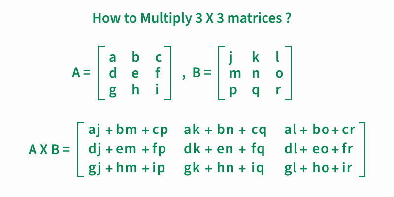
(Figure 5. Example of matrix multiplication)

(Table 1: Energy consumption of BitNet and Transformer varying different model size. Results are reported with 512 as input length.)

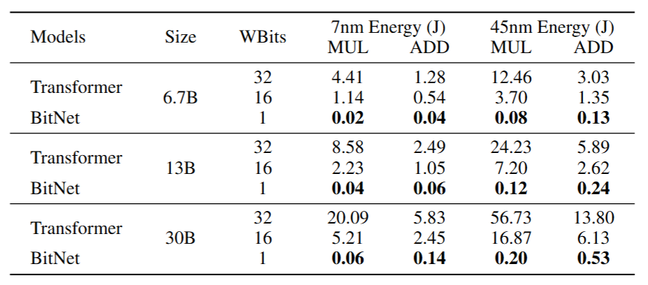
(Table 2. ADD and MUL energy consumption for different bit representations at 45nm and 7nm process nodes)

Comparison with FP16 transformers

Setup

• Train a series of autoregressive language models with BitNet of various scales, ranging from 125M to 30B
• The models are trained on English-language corpus, which consists of the Pile dataset, Common Crawl snapshots, RealNews, and CC-Stories dataset
• Also train the transformer baselines with the same datasets and settings for a fair comparison

Neural language models have proven to scale predictably with vanilla transformer

• The loss scales as the power law with the amount of computation for training
• This allows us to determine the optimal allocation of a computation budget as well as predict the performance from the size of models
• $L(N) = aN^b+c$

Scaling law between loss and model size

• The loss scaling of BitNet is similar to the Floating Point(FP)FP16 transformer, which follows a power-law
• The gap between BitNet and FP16 transformer becomes smaller as the model size grows

Inference-optimal scaling law

• Predicts the loss against the energy consumption
• Scaling curve against the inference energy cost at 7nm process nodes
• BitNet has much higher scaling efficiency

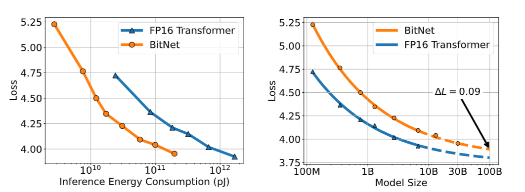
(Figure 6: Scaling curves of BitNet and FP16 Transformers)

Results on downstream tasks

• Test both the 0-shot and 4-shot results on four downstream tasks, including Hellaswig, Winogrande, Winogrand, and Storycloze for evaluate the capabilities (see Appendix for more details about benchamark datasets)
• The performance on the downstream tasks can scale as the computation budget grows
• The scaling efficiency of capabilities is much higher than the FP16 transformer baseline

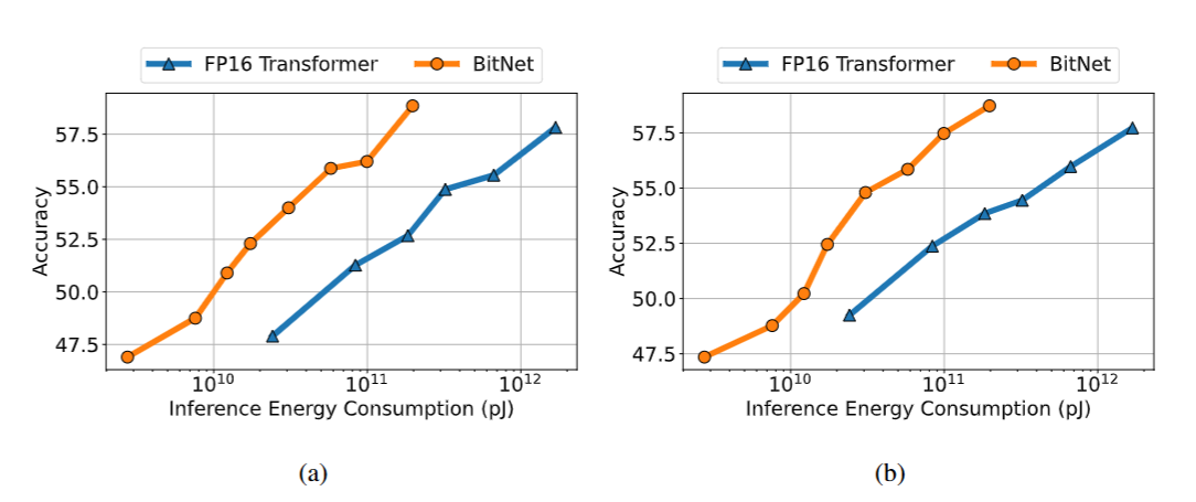
(figure 7. Zero-shot (Left) and few-shot (Right) performance of BitNet and FP16 Transformer against the inference cost.)

Stability test

• BitNet can converge with a large learning rate while FP16 transformer can not, demonstrating better training stability of BitNet, enables the training with larger learning rates

• BitNet can benefit from the increase in learning rate, achieving better convergence in terms of PerPLexity(PPL)

\[Perplexity(W) = P(w_1, w_2, ..., w_N)^{-\frac{1}{N}} = \exp\left(-\frac{1}{N}\sum_{i=1}^N \log P(w_i|w_1,...,w_{i-1})\right)\]

• Lower perplexity indicates that the model is better at predicting the next word in a sequence, while a higher perplexity means more uncertainty and poorer prediction

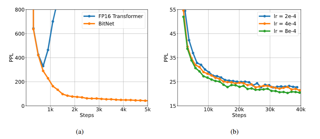
(Figure 8. BitNet is more stable than FP16 Transformer with a same learning rate (Left). The training stability enables BitNet a larger learning rate, resulting in better convergence (Right))

Comparison with post-training quantization

Setup

• Compare BitNet with state-of-the-art quantization methods, including Absmax, SmoothQuant, Generative Pre-trained Transformer Quantized(GPTQ), and Quantization with Incoherence Processing(QuIP)
  • These are post-training quantization over an FP16 transformer model
  • Absmax and SmoothQuant quantize both the weights and the activations, while GPTQ and QuIP only reduce the precision of weights
• Experiment with W4A16 and W2A16 for the weight-only quantization(GPTQ and QuIP)
• Experiment with W8A8, W4A4, and W1A8 for the weight-and-activation quantization(Absmax and SmoothQuant)
• BitNet is binary weight 8-bit activation(W1A8)
• Evaluate on four benchmark dataset, Winogrande, Winograd, Storycloze, and Hellaswag

Results

• Demonstrate the effectiveness of BitNet in achieving competitive performance levels compared to the baseline approaches
• Advantage is consistent across different scales

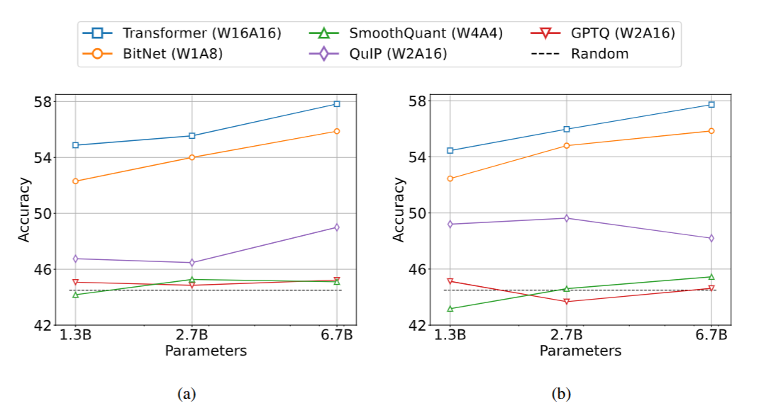
(Figure 9. Zero-shot (Left) and few-shot (Right) results for BitNet and the post-training quantization baselines on downstream tasks.)

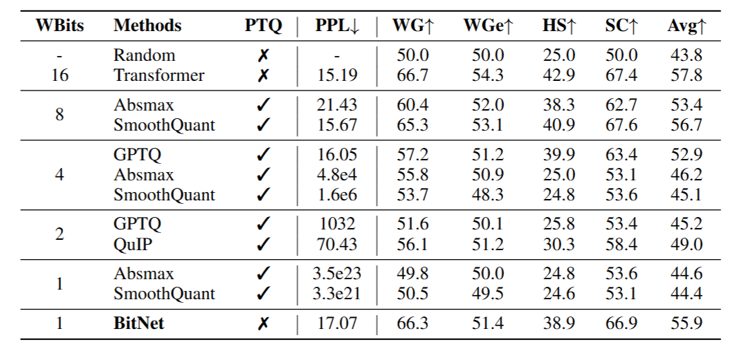
(Table 3. Zero-shot results for BitNet and the baselines (PTQ: Post-training quantization, WGe: Winogrande, WG: Winograd, SC: Storycloze, and HS: Hellaswag dataset).)

Ablation Studies

Effect of choices in activation quantization as well as the techniques to stabilization

• In experiments, absmax has better performance and makes training more stable than elastic(Liu et al., 2022)
• Elastic dynamically adjusts the scales with learnable parameters
• SubLN outperforms both Pre-LN and Binarized neural Machine Translation(BMT)(Zhang et al., 2023)
  • Pre-LN is the default architecture of Generative Pre-trained Transformer(GPT)
  • BMT has proven to improve the stability of binarized models

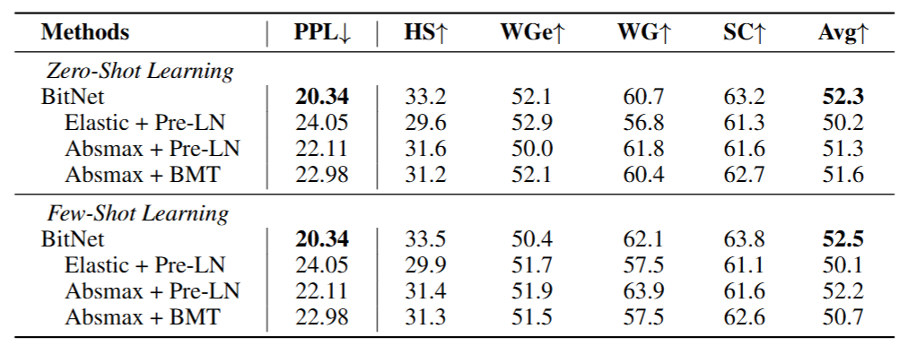
(Table 4: Ablation of BitNet (WGe: Winogrande, WG: Winograd, SC: Storycloze, and HS: Hellaswag dataset). Elastic is an activation quantization method from (LOP+22 ), while BMT is the architecture from (ZGC+23) to stabilize the training of low-bit models.)

Conclusion and Future Works

• BitNet, a novel 1-bit transformer architecture for large language models Designed to be scalable and stable, with the ability to handle large language models efficiently

• The experimental results demonstrate that BitNet achieves competitive performance in terms of both perplexity and downstream task performance, while significantly reducing memory footprint and energy consumption

• BitNet follows a scaling law similar to that of full-precision transformers, indicating that it can be effectively scaled to even larger language models

• In the future, we would like to scale up BitNet in terms of model size and training steps

Appendix

Parameters of GPT-3

As the size of the parameter increases, the parameters of FFN and Multi-head Attentions take up the majority of the total parameters

see Effecitve GPT-3(175B): GPT-3 파라미터 요구사항 계산과 분석

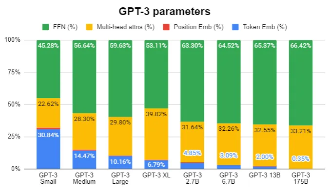
(Figure 10. GPT-3 parameters component by model size)

Variance and expectation

The definition of variance is a metric that indicates how far a random variable is from its expected value.

\[Var(x) = E\left[(x-E(x))^2\right] = E[x^2 - 2xE[x] + E[x]^2] = E[x^2] - 2E[xE[x]] + E[E[x]^2] \\ \text{Since } E[x] \text{ is constant, } E[xE[x]] = E[x]E[x] = E[x]^2, \text{ and } E[E[x]^2] = E[x]^2 \\ \therefore Var(x) = E[x^2] - E[x]^2\]

Weights Initialization

Kaiming initialization

\[\textbf{W} = N(0, \frac{2}{n})\]

Xavier initialization

\[\textbf{W} = N(0, \frac{1}{n})\]

Derivation of $E[|W|] \approx \sigma = \frac{1}{\sqrt{n}}$

Note that average of W is almost 0

\[E[|W|] = \int_{-\infty}^{\infty} |w| \frac{1}{\sigma\sqrt{2\pi}} \exp\left(-\frac{w^2}{2\sigma^2}\right) dw \\ \text{Since it is even, } E[|W|] = 2 \int_{0}^{\infty} w \frac{1}{\sigma\sqrt{2\pi}} \exp\left(-\frac{w^2}{2\sigma^2}\right) dw \\ \text{By substitution } u = \frac{w^2}{2\sigma^2} \left(du = \frac{w}{\sigma^2} dw\right), E[|W|] = 2 \int_{0}^{\infty} w \frac{1}{\sigma\sqrt{2\pi}} \exp(-u) \frac{\sigma^2}{w} du \\ 2 \int_{0}^{\infty} w \frac{1}{\sigma\sqrt{2\pi}} \exp(-u) \frac{\sigma^2}{w} du = 2 \frac{\sigma}{\sqrt{2\pi}} \int_{0}^{\infty} \exp(-u) du = \frac{2\sigma}{\sqrt{2\pi}} = \sigma \sqrt{\frac{2}{\pi}} \approx 0.7979\sigma\]

Since GPT-3 175B has size of 12288 feature dimension(n=12288), standard deviation is very low($\sigma \approx 0.01$)

\[\therefore E[|W|]=0.7979\sigma \approx \sigma = \frac{1}{\sqrt{n}}\]

Note that initial variance of $W$ is $\frac{1}{\sqrt{n}}$, this variance can be changed during training.

However, GPT-3 small has size of 768 feature dimension (n=768), 𝜎=0.03 and still low but this is cause of gap between FP16 transformer and BitNet at small model size

Despite the average of W can be changed during training, average of W is so small that it’s negligible(the average of weight is -0.01 to 0.01 in pre-trained GPT2) because of Weight decay

if average is not zero…

\[E[|X|] = \mu \cdot (2\Phi(\frac{\mu}{\sigma}) - 1) + \sigma \cdot \sqrt{\frac{2}{\pi}} \cdot \exp(-\frac{\mu^2}{2\sigma^2})\]

where $\Phi(z)$ is cumulative distribution function (CDF) of the standard normal distribution

if $\mu \gg \sigma$, expectation of absolute value is almost $\mu$.

if $\mu \ll \sigma$, and $\mu$ is almost zero, expectation of absolute value is almost $\sigma \cdot \sqrt{\frac{2}{\pi}}$

if $\mu == \sigma,$ expectation of absolute value is \(\sigma \cdot (2\Phi(1) - 1) + \sigma \cdot \sqrt{\frac{2}{\pi}} \cdot \exp(-0.5)\)

\[=\sigma \cdot (2 \cdot 0.84134 - 1) + 0.6065\cdot \sigma \sqrt{\frac{2}{\pi}} \approx 1.03\sigma\]

however, in BitNet, $\mu$ is not much bigger than $\sigma$, therefore we can ignore the $\mu$

Quantizaiton

• Per-tensor quantization
  • Apply a single scaling factor across an entire tensor, offering computational efficiency but potentially lower accuracy when values vary widely
• Per-token quantization
  • Apply different quantization parameters for each token, allowing for more precise representation of varying data distributions

Norm

\[\text{1-norm } \|x\|_1 = \sum_{i=1}^n |x_i|\] \[\text{2-norm } \|x\|_2 = \sqrt{\sum_{i=1}^n x_i^2}\] \[\infty\text{-norm } \|x\|_{\infty} = \max_i |x_i|\]

Why $\text{Var}(y) = n\text{Var}(wx)$

In a neural network, the output $y$ is typically computed as a sum of products

\[y=\sum_{i=1}^n w_i x_i\]

According to probability theory, when we have independent random variables, the variance of their sum equals the sum of their variances

\[\text{Var} (\sum_{i=1}^n X_i) = \sum_{i=1}^n \text{Var}(X_i)\]

If we asuume each term $w_ix_i$ has the same variance, and all terms are independent, then \(\text{Var}(y) = \text{Var} (\sum_{i=1}^n w_ix_i) = \sum_{i=1}^n \text{Var}(w_ix_i) = n\cdot \text{Var}(wx)\)

‘n’ represent the number of independent terms being summed together, which typically corresponds to the number of input neurons or features in the network

Benchmark datasets

• Winogrande(Sakaguchi et al., 2021)
  • A benchmark for commonsense reasoning, with a set of 273 expert-crafted pronoun resolution problems
• Winograd(Levesque et al., 2012)
  • A benchmark for commonsense reasoning

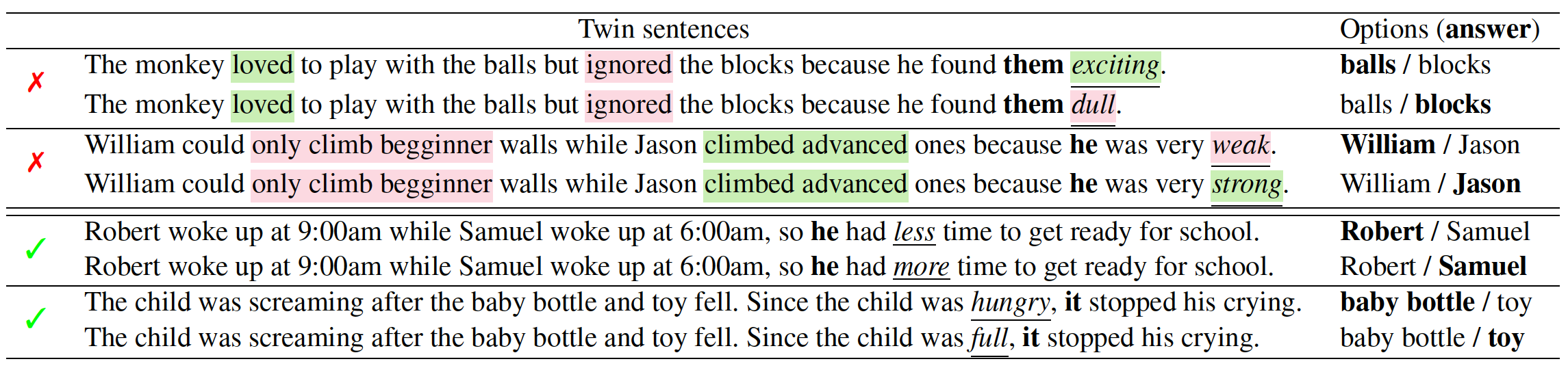
(Figure 11. Example data of Winogrande)

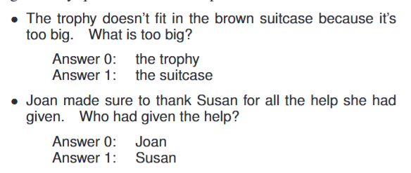
(Figure 12. Example data of Winograd schema challenge)

• Storycloze(Mostafazadeh et al., 2016)
  • A benchmark for narrative commonsense reasoning, with a set of 3744 stories
• Hellaswag(Zellers et al., 2019)
  • A benchmark for commonsense reasoning and contextual suitability with a set of about 10,000 problems collected from Activitynet and Wikihow

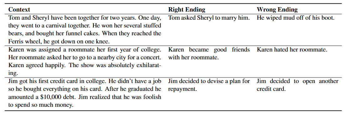
(Figure 13. Three example Story Cloze Test cases, completed by our crowd workers.)

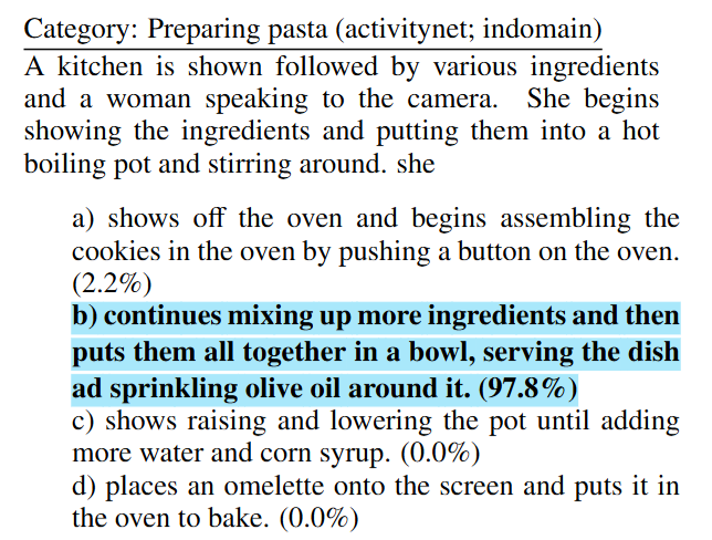
(Figure 14. Example HellaSwag questions answered by BERT-Large. Correct model predictions are in blue, incorrect model predictions are red. The right answers are bolded.)

Elastic

• Introduced in “BiT: Robustly Binarized Multi-distilled Transformer”
• Binarizes weights to (-1,1) and ReLU/Softmax output to (0,1) with an elastic binarization function using learnable parameters
• Multi-distillation approach that gradually transfers knowledge from higher-precision models to lower-precision ones

Post-LN

• Standard Transformer layer

\[h'= LN(h+Attention(h)) \\ o=LN(h'+FFN(h'))\]

Pre-LN

\(h'=h+Attention(LN(h)) \\ o=h'+FFN(LN(h'))\)

BMT

• Adds extra layernorm operation to dynamically normalize the outputs of binarized layer
• Adds extra shortcut connections around output projection layer in attention mechanisms
• This approach helps stability of binarized transformer

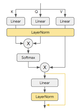
(Figure 15. BMT Multi-Head Attention — Differences from the original Transformer are highlighted (in yellow). All linear projections and einsums can be binarized )