Effective Approaches to Attention-based Neural Machine Translation

paper-review

This article is review of Luong et al., Effective Approaches to Attention-based Neural Machine Translation

Introduction

• Neural Machine Translation(NMT) achieved state-of-the-art performances in large-scale translation tasks

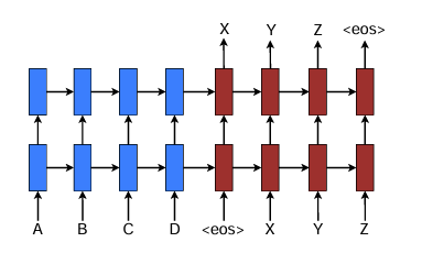
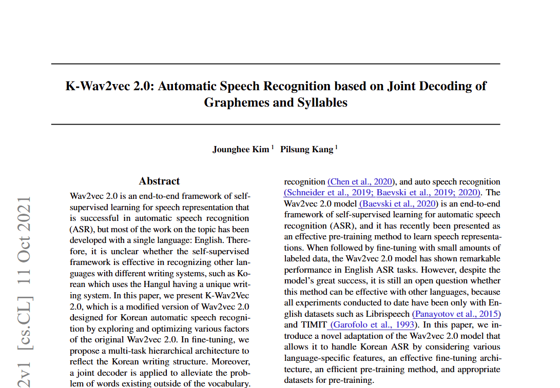
(Figure 1. Neural machine translation - a stacking recurrent architecture for translating a source sequence A B C D into a target sequence X Y Z. Here, eos marks the end of a sentence)

• Typical NMT uses sequence-to-sequence model.
• sequence-to-sequence model consists of encoder and decoder
• In figure 1, the encoder and the decoder is 2-layer LSTMs each
  • This means that the first layer receive embedded text and previous hidden state of first layer as input, and the second layer receive output of first layer and previous hidden state of second layer as input
  • The output of decoder is translated result
  • The encoder encoded the original text and final hidden vector is fed into decoder as source sentence representation
  • The decoder predict next word probability using previous hidden state and previous predicted word
    • with eos as input, decoder predict the first word(X)
    • with first word(X) as input, decoder predict the second word(Y)
  • Sequence-to-sequence model is trained with Teacher forcing
    • Teacher forcing is that the predicted output of the decoder cell from the previous is not input to the decoder cell from the current, but the real(target) value from the previous is used as the input value of the decoder cell from the current
• In parallel, the concept of attention has gained popularity recently in training neural networks, allowing models to learn alignments between different modalities, e.g., between speech frames and text in the speech recognition, or between picture and its text description
• In the context of NMT,Bahdanau et al. (2015) has successfully applied such attentional mechanism to jointly translate and align words.
• In this work, we design, with simplicity and effectiveness in mind, two novel type of attention based models: a global approach in which all source words are attended and a local one whereby only a subset of source words are considered at a time

Neural Machine Translation

A neural machine translation system is a neural network that directly models the conditional probability $ p(y|x) $ of translating a source sentence, $ x_1,…, x_n $ to a target sentence, $ y_1,…,y_m $. The conditional probability is

\[\log p(y|x)=\sum_{j=1}^{m} \log p(y_j|y_{<j}, \textbf{s})\]

,where $s$ is the source representation of encoder

• In previous works, RNN, LSTM, GRU and CNN was used for encoder, and RNN, LSTM and GRU was used for decoder
• Probability of word $y_i$ is calculated from current hidden state(with weight $W$):

\[p(y_i|y_{<j},\textbf{s}) = softmax(g(\textbf{h}_j ))\]

• outputs of g function are vocabulary-sized vector.

$\textbf{h}_j $ is the RNN hidden unit, abstractly computed as

\[\textbf{h}_j=f(\textbf{h}_{j-1},\textbf{s})\]

$f$ computes the current hidden state given the previous hidden state(+ usually with previous output as current input)

In Kalchbrenner and Blunsom, 2013, Sutskever et al., 2014, Cho et al., 2014, Luong et al., 2015, the source representation $\textbf{s}$ is only used once to initialize the decoder hidden state

On the other hand, in (Bahdanau et al., 2015, Jean et al., 2015), and this work, $\textbf{s}$ implies a set of source hidden states(encoder hidden states) which are referred throughout the entire course of the translation(decoding) process.

In this paper, the author uses the 2-layer LSTM architecture.

Training objective is

\[J_t=\sum_{(x,y)\in D} - \log p(y|x)\]

with D being parallel training corpus, $ x $ being input sentence, $ y $ being target sentence. The higher the probability the model gives the correct answer, the smaller the log value

By minimizing the sum of these values in all training data, the performance of the model is improved.

Attention-based model

Attention models are classified into global and local.

these models differ in how the context vector $c_t$ is derived. context vector $c_t$ captures relevant source-side(encoder-side hidden state) information to help predict the current target word $y_t$.

Attentional hidden state is produced as follows

\[\tilde{\textbf{h}}_t = \tanh (W_c[\textbf{c}_t;\textbf{h}_t])\]

, with concatenating the context vector and hidden state

The attentional hidden state is then fed through the softmax layer to produce the predictive distribution formulated as

\[p(y_t|y_{<t},x)=softmax(\textbf{W}_s \tilde{\textbf{h}}_t)\]

Global Attention

Consider all the hidden states of the encoder when deriving the context vector.

align vector $\textbf{a}_t(s)$ indicates the proportion of attention that the decoder’s hidden vector at time step $t$ should pay to the encoder’s hidden vector at position $s$ among all encoder hidden vectors

\[\textbf{a}_t(s) = align(\textbf{h}_t, \textbf{h}_s)=\frac{\exp (\textbf{score}(\textbf{h}_t, \textbf{h}_s))}{\sum_{s'}\exp (\textbf{score}(\textbf{h}_t, \textbf{h}_{s'}))}\]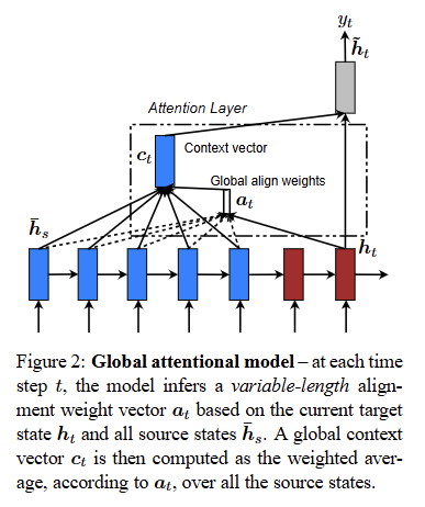

score function indicates that how much attention the hidden vector at time $t$ on the decoder should pay to $s$ hidden vector on the encoder

there are 3 different alternatives score function.

first is $dot$ score function

\[\textbf{score}(\textbf{h}_t, \textbf{h}_s)= \textbf{h}_t^\top \textbf{h}_s\]

second is $general$ score function

\[\textbf{score}(\textbf{h}_t, \textbf{h}_s)= \textbf{h}_t^\top \textbf{W}_a\textbf{h}_s\]

third is $concat$ score function

\[\textbf{score}(\textbf{h}_t, \textbf{h}_s)= \textbf{v}_a^\top\tanh(\textbf{W}_a[\textbf{h}_t ;\textbf{h}_s])\]

, where $\textbf{v}_a$ and $\textbf{W}_a$ are learnable parameters

The authors also attempts to use $location-based$ function in which the alignment scores are computed from solely the decoder’s hidden state

\[\textbf{a}_t = softmax(\textbf{W}_a \textbf{h}_t)\]

Given the alignment vector as weights, the context vector is computed as the weighted average over all the source hidden states in each top layer of encoder $E$

\[\textbf{c}_t=\sum_{i \in E} \textbf{a}_t(i)\textbf{h}_i\]

Local Attention

The global attention ahs a drawback that it has to attend to all words on the source(encoder) side for each target word, which is expensive and can potentially render it impractical to translate longer sequences

The author proposes a local attention mechanism that chooses to focus only on a small subset of the source positions per target word.

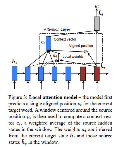
The local attention mechanism selectively focuses on a small window of context and is differentiable.

The model first generates an aligned position $p_t$ for each target word at time $t$. The context vector $c_t$ is then derived as a weighted average over the set of source hidden states within the window $[p_t−D, p_t+D]$. $D$ is empirically selected.

Unlike the global approach, the local alignment vector $\textbf{a}_t$ is now fixed-dimensional, i.e., size of window $R^{2D+1}$. The authors consider two variants of the model as below

$Monotonic$ alignment (local-m): simply set $p_t=t$, assuming that source and target sequences are roughly monotonically aligned. The alignment vector $\textbf{a}_t$ is defined same as global attention. this means that the word at position $t$ in source sentence appears at position $t$ in target sentence.

$Predictive$ alignment (local-p): The model predicts an aligned position(i.e., the encoder hidden state aligned with the decoder time step $t$) as follows

\[p_t = S\cdot sigmoid(\textbf{v}_p^\top \tanh (\textbf{W}_p \textbf{h}_t))\]

$\textbf{v}_p$ and $\textbf{W}_p$ are the learnable parameters(model parameters). and $S$ is the source sentence length. Since output of sigmoid function is in 0 to 1, $p_t \in [0,S]$

Alignment weights are now defined as

\[\textbf{a}_t = align(\textbf{h}_t, \textbf{h}_s) \exp -(\frac{(s-p_t)^2}{2\sigma^2})\]

align function is same as in global attention, and the standard deviation $\sigma$ is empirically set as $\frac{D}{2}$

By multiplying exp term, we can pay more attention to aligned position.

Input-feeding approach

In above global and local attention, the attentional decisions are made independently(the model can’t recognize the previous attentional decision and attentional hidden state).

Whereas, in standard machine translation, a coverage set is often maintained during the translation process to keep track of which source words have been translated.

Likewise, in attentional NMTs, alignment decisions should be made considering the past alignment(attention) information

To address that, the authors propose an input-feeding approach in which attentional vectors $\tilde{h}_t$ are concatenated with inputs at the next steps

\[input_{cur} = [\tilde{h}_{prev};output_{prev}]\]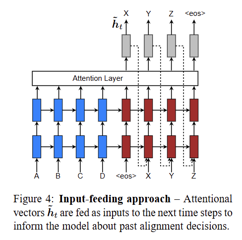

In figure 4, input is concatenation of previous attentional vector $\tilde{h}_t$ and previous output $X$

Experiments

Evaluate the effectiveness of the models on the WMT translation tasks between English and German in both directions

performances are reported in case-sensitive BLEU on newstest2014 and 2015.

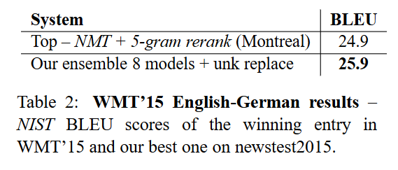
quality are reported in two types of BLEU, tokenized BLEU and NIST BLEU.

BLEU measure how many n-grams appear in the machine translation result are included in the reference.

In Case sensitive BLEU, ‘The’ and ‘the’ is different word.

Tokenized BLEU measure the BLEU based on the tokenized text

The cat's toy is red.

(the, cat, 's, toy, is, red, .)

In NIST BLEU, rare n-grams are considered more important information and give higher scores

Training details

• All models are trained on the WMT 14 training data consisting of 4.5M sentences pairs with 116M English words and 110M German words

• Limit vocabularies to be the top 50k most frequent words for both languages.
  • Words not in these shortlisted vocabularies are converted into a universal token
• Stacking LSTM models have 4 layers, each with 1000 cells, and 1000-dimensional embeddings

import tensorflow as tf
from tensorflow.keras.models import Sequential
from tensorflow.keras.layers import LSTM, Dense
model = Sequential()
model.add(LSTM(1000, return_sequences=True, input_shape=(100, 1000)))
model.add(LSTM(1000, return_sequences=True))
model.add(LSTM(1000, return_sequences=True))
model.add(LSTM(1000))

• Empirically set the window sizeD = 10.

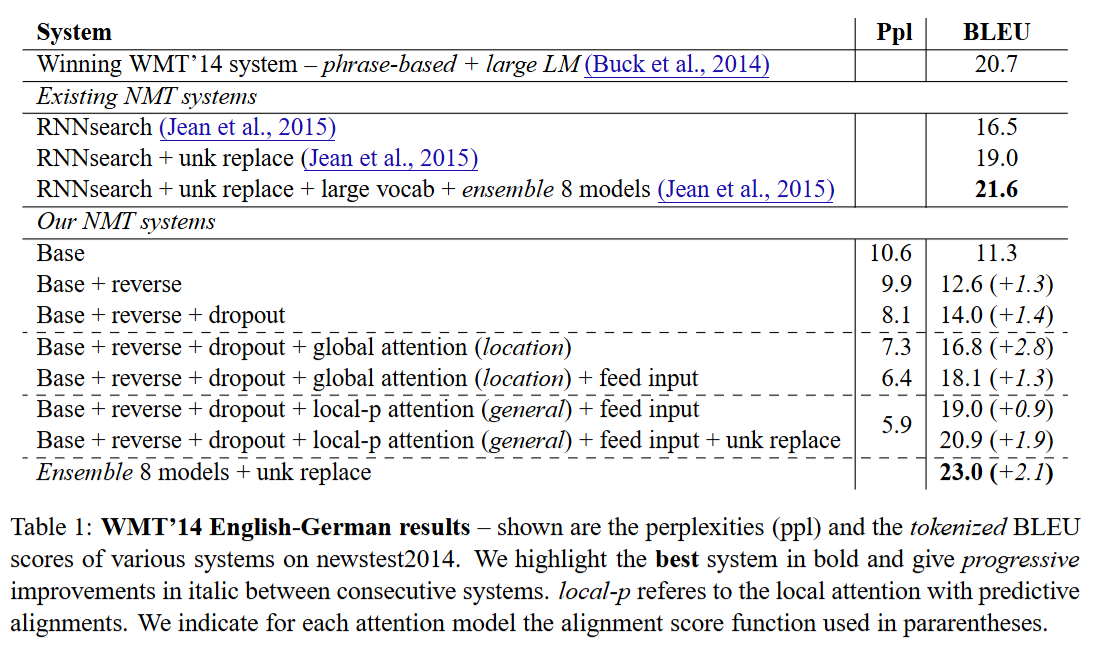
English-German Results

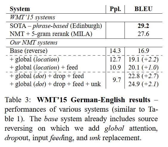
German-English Results

Analysis

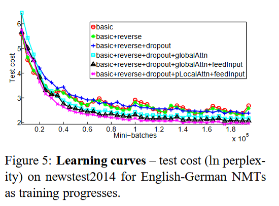
Learning curves

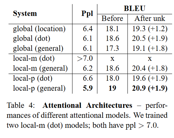
Perplexity(ppl) is a metric that measures how well a language model predicts next token based on previous words

\[PPl = \exp (-\frac{1}{N} \sum_{i=1}^N \log P(w_i | w_1, ..., w_{i-1}))\]

Lower perplexity means the model is more confident and accurate in its prediction.

For example, perplexity is low if the model predicts ‘apple’ as 95% and ‘melon’ as 5%. On the other hands, it is high if the model predicts ‘apple’ as 55% and ‘melon’ as 45%.

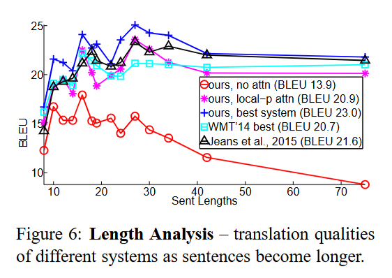
Effects of Translating Long Sentences

Choices of Attentional Architectures

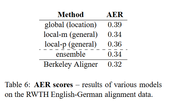
Alignment Quality

Evaluate the alignment quality using the alignment error rate (AER) metric

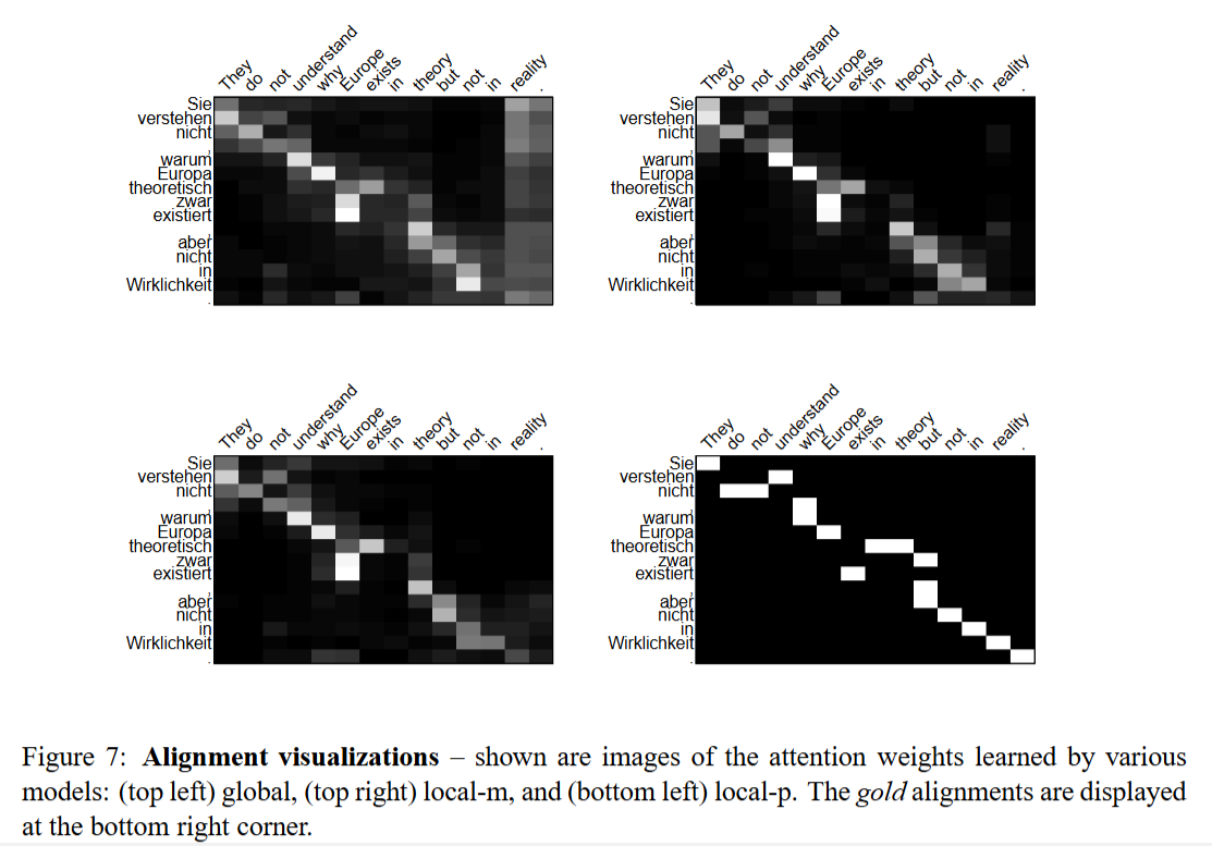
Decoding attentional status between words in English sentences and words in German sentences

Conclusion

• propose two simple and effective attentional mechanisms for neural machine translation: global attention and local attention

• local attention yields large gains of up to 5.0 BLEU over non-attentional models