
MobileNets: Efficient Convolutional Neural Networks for Mobile Vision Applications
paper review
This article is review of Howard et al., MobileNets: Efficient Convolutional Neural Networks for Mobile Vision Applications. 2017
Introduction
Primary trend
- Convolutional Neural Networks(CNN) have become ubiquitous in computer vision
- Making deeper and more complicated networks
- Improving accuracy
- Not necessarily making more efficient with size and speed
- Many applications need to be carried out in restricted environment
This paper
- Describing Mobilenet, an efficient network architecture
- Building smaller, lower latency model with two hyper parameters
- Matching requirements for mobile and embedded vision
Prior work
Flattened CNN
- Replacing $C\times X\times Y$ filters with
- $C\times 1 \times 1$ lateral filters
- $1\times Y \times 1$ vertical filters
- $1\times 1\times X$ horizontal filters
- Advantages
- Parameters are reduced from $C\times X\times Y$ to $C + X + Y$
- Accelerating feedforward and backward computation of CNNs
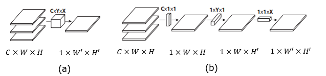
(Figure 1. (a) CNN operation (b) Flattened CNN operations)
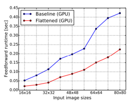
(Figure 2. Comparison of execution time between baseline and flattened model)
SqueezeNet
- Bottleneck approach to design small network
- Achieves comparable performance to AlexNet while reducing parameters by 50x
- Squeeze convolution layer compressing channel dimension with 1×1 convolutional layers
- Expand convolution layer expanding channel dimension with 1×1 and 3×3 convolutional layers
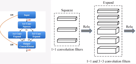
(Figure 3. A block consisting SqueezeNet)
Distillation
- Transferring knowledge of large models to one small model
- Large models produce soft targets
- Softmax probability distribution using logits divided by $T$
- Helps transfer knowledge about similarities between classes
- A small model learns from both probability distribution and true labels
- Smaller model size while maintains similar accuracy to large model
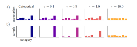
(Figure 4. probability distribution by T)
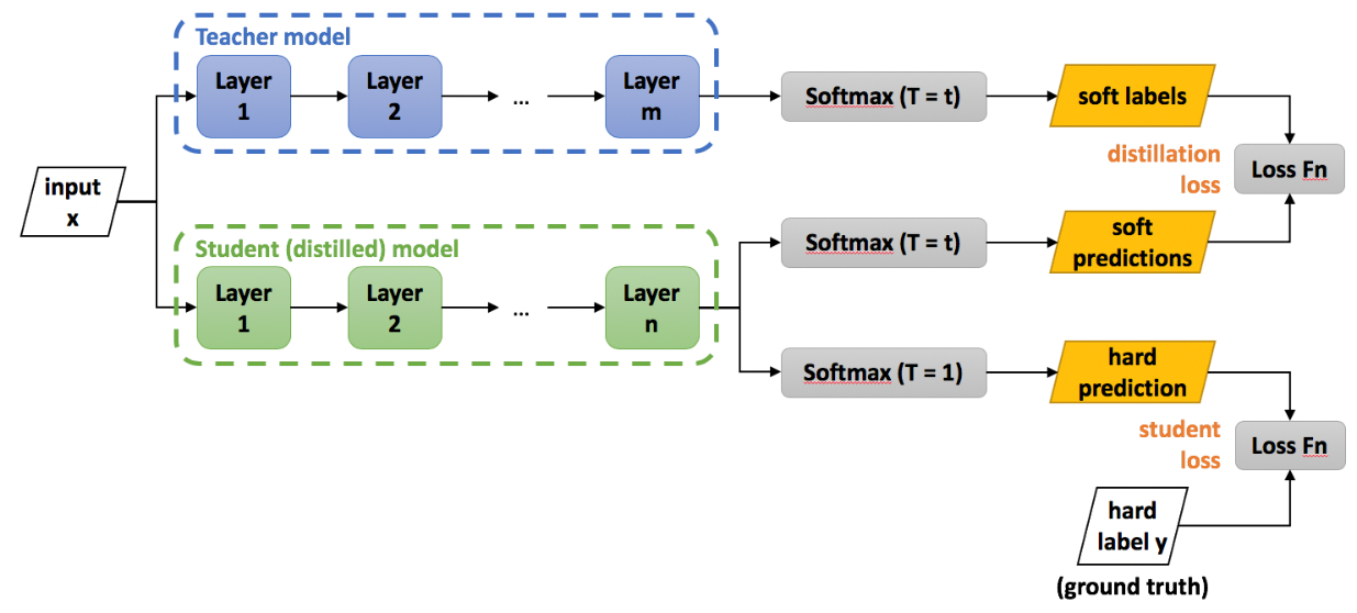
(Figure 5. The architecture of knowledge distillation)
MobileNet architecture
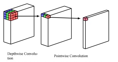
- Factorizing convolution layer into depthwise separable filter
- Depthwise separable filter consists of Depthwise convolution layer and Pointwise convolution layer
- MobileNet consists of 1 convolutional layer, 13 depthwise separable filter, 1 $7\times 7$ average pooling, which reduce feature map $C\times 7\times 7$ to $C\times 1 \ times 1$, and 1 fully connected layer with 1000 classes
- Shrinking parameter of baseline MobileNet
- Width multiplier reduce input channel dimension
- Resolution multiplier reduce input resolution
Depthwise separable convolution
- Factorize a standard convolution into depthwise convolution and pointwise convolution
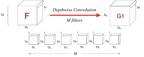
Depthwise convolution
- Perform spatial convolution independently on each input channel
- Extract feature without channel information combination
- Channel dimensions are remained
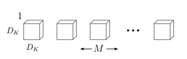
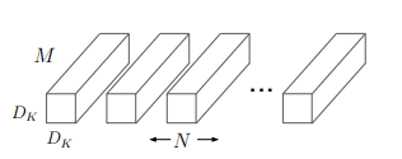
- For $M\times D_F \times D_F$ input feature map, there are $M$ of $ 1\times D_k \times D_k$ filters
(Figure 6. Depthwise separable convolution )
(Figure 7. Depthwise convolution filters)
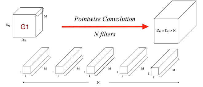
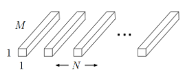
Pointwise convolution
- uses $M\times 1\times 1$ convolution to combine across channels : $M\times W\times H$ input to $1\times W\times H$
- combine the output the depthwise convolution
- From $M\times D_G\times D_G$ input, there are $ N $ of $ M\times 1\times 1$ filters for $N\times D_G \times D_G$ output
(Figure 8. Pointwise convolution)
Computational cost of depthwise separable convolution layer
Depthwise convolution layer
- Assuming a single filter per each input channel
Therefore the cost is
\[D_k \times D_k \times M \times D_F \times D_F\]- because each convolution costs $D_k\times D_k$ multiplication and this multiplication applied to each position in the $D_F\times D_F$ in one channel. Also, there are $M$ filters because there are $M$ channels
Pointwise convolution layer
The cost is
\[M\times N\times D_F\times D_F\]- because $M$ channel combination into one channel costs $M$, and this channel combination applied to each position in the $D_F\times D_F$ feature maps. Also $M$ channel combination reply $N$ times to produce $N$ channel output
(Figure 9. Depthwise convolution filter)
(Figure 10. Pointwise convolution filter)
Comparison between standard and depthwise separable convolution
Costs of standard convolution is \(D_K \times D_K \times M \times N \times D_F \times D_F\)
Costs of depthwise separable convolution is
\[D_k \times D_K \times M \times D_F \times D_F + M \times N \times D_F \times D_F\]Reduction in computation of
\[\frac{D_k \times D_K \times M \times D_F \times D_F + M \times N \times D_F \times D_F}{ D_K \times D_K \times M \times N \times D_F \times D_F} = \frac{1}{N} + \frac{1}{D_K^2}\]Since MobileNet uses $3\times 3$ depthwise separable convolutions, It costs 8 to 9 time less computation than standards
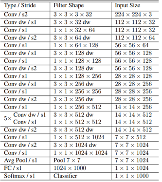
Network structure and training
(Table 1. MobileNet architecture)
-
MobileNet consists of 1 convolutional laer, 13 depthwise separable filter, 1 $7\times 7$ average pooling, and 1 fully connected layer with 1000 classes
-
depthwise separable filter consist of 1 $3\times 3$ depthwise convolution filter and 1 $1\times 1$ pointwise convolution filter
-
All layers except final fully connected layer are followed by batch normalization, Rectified Linear UNit(ReLU)
- Downsampling is handled with strided convolution
- Trained in Tensorflow using Root Means Square PROPagation(RMSProp)
Multipliers
- MobileNets construct MobileNet smaller and less computationally expensive
Width multipliers
-
parameter $\alpha$ where \(0 < \alpha \leq 1\)
-
Thin a network uniformly at each layer. The number of input channel $M$ becomes $\alpha M$, and the number of output channel $N$ becomes $\alpha N$.
-
Computational costs are \(D_k \times D_K \times \alpha M \times D_F \times D_F + \alpha M \times \alpha N \times D_F \times D_F\)
-
Kernel size are
- Reducing computational cost and number of parameters by roughly $\alpha ^2$
Resolution multipliers
-
parameter $\rho$ where \(0 < \rho \leq 1\)
- Reduce an input image and internal representation of every layer
- Input image resolution $M\times D_F \times D_F$ becomes $M\times \rho D_F \times \rho D_F$
- Output feature map resolution $N\times D_G \times D_G$ becomes $N \times \rho D_G \times \rho D_G$
- Computational cost
- Reducing only computational cost by $\rho ^2$
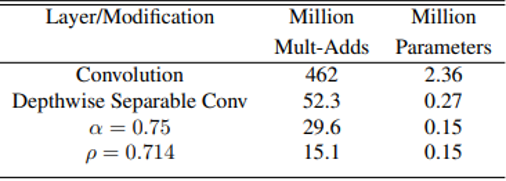
(Table 2. Resource usage for modification to standard convolution. Each row is a cumulative effect adding on top of the previous row. Input feature map of size 14 x 14 x 512 with kernel size of 3 x 3 x 512 x 512)
Experiments
Model choices
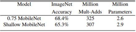
- MobileNet with depthwise separable versus full convolution
- Depthwise separable convolutions reduces accuracy by 1 percent on ImageNet While saving tremendously on mult-adds and parameters
- thinner model versus shallower model
- Thinner model uses width multiplier 0.75
- Change input, output channel 32, 64 to 24, 48
- In the shallower model, the 5 layers of separable filters are removed
- Thinner MobileNet is 3 percent better than making shallower while shows similar computation and number of parameters
- Thinner model uses width multiplier 0.75
(Table 3. Depthwise separable vs full convolution MobileNet)
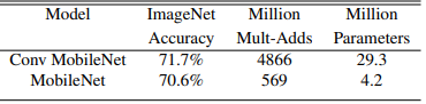
(Table 4. Narrow vs shallow MobileNet)
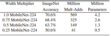
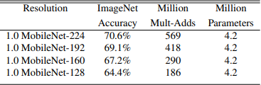
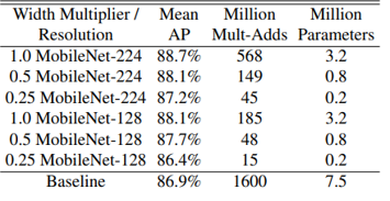
Model shrinking hyperparameters
Width multiplier
- Mult-adds and parameters decreases in proportion of roughly $\alpha ^2$
- Accuracy drops smoothly until $\alpha = 0.25$
Resolution multiplier
- Mult-adds decreases in proportion of roughly $\rho ^2$
- The number of parameters are same because kernel size are same
- Accuracy drops off smoothly across resolution
(Table 5. MobileNet width multiplier)
(Table 6. MobileNet resolution multiplier)
shrinking hyperparameters experiments
- 16 models made from the cross product of Width multiplier $\alpha \in {1,0.75,0.5,0.25}$ and input image resolution ${ 224, 192, 160, 128}$.
- Trade off between computation and ImageNet accuracy
- Log linear with a jump when models get very small at $\alpha = 0.25$.
- Trade off between number of parameters and ImageNet accuracy
- Accuracy drops smoothly except for nearly 0.4 million
- The number of parameters do not vary based on the input resolution
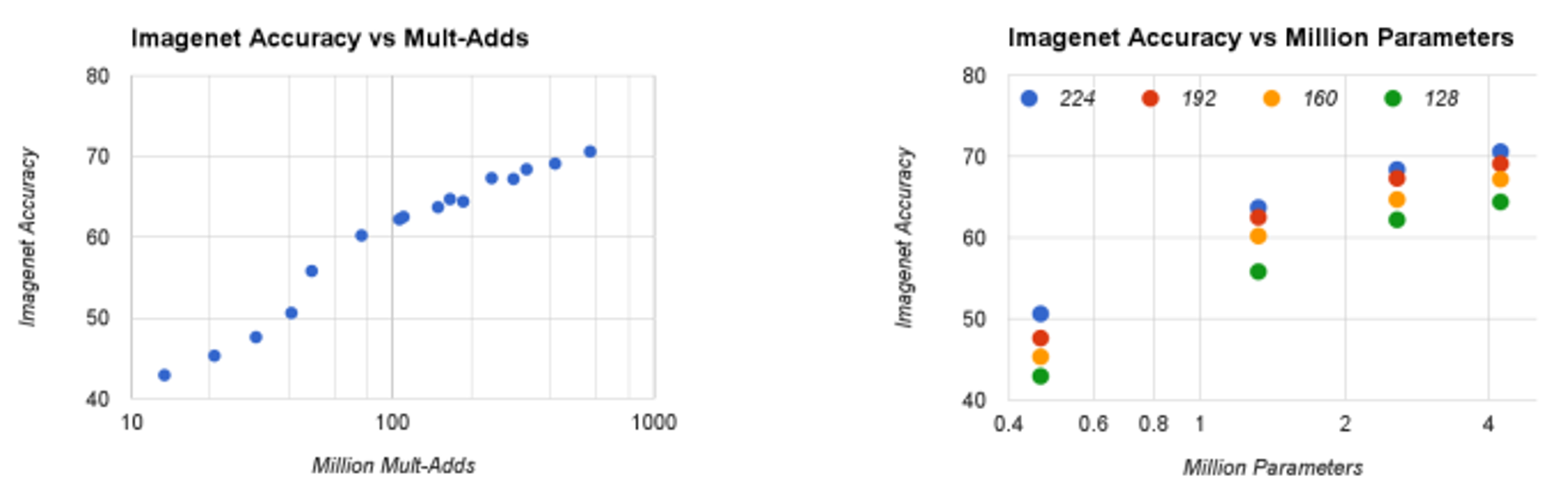
(Figure 11. (a)Trade off between computation and accuracy (b)trade off between number of parameters and accuracy)
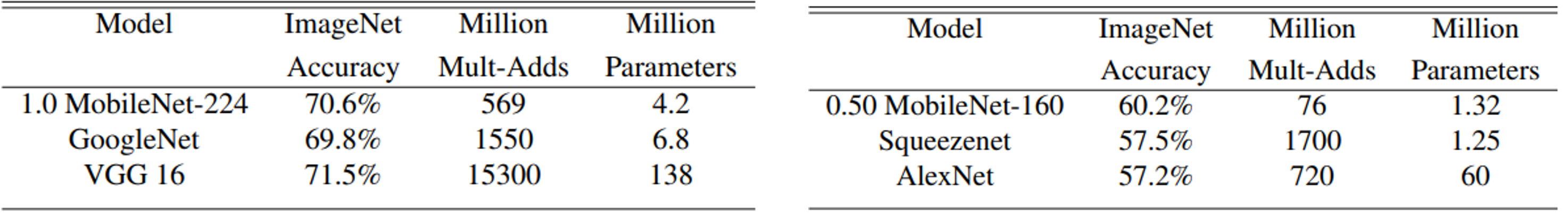
MobileNet comparison to other models
- MobileNet with 𝛼=1.0 and input resolution is 224
- Nearly as accurate as Visual Geometry Group(VGG)16 while being 32 times smaller and 27 times less compute intensive
- More accurate than GoogleNet, while being smaller and more than 2.5 times less computation
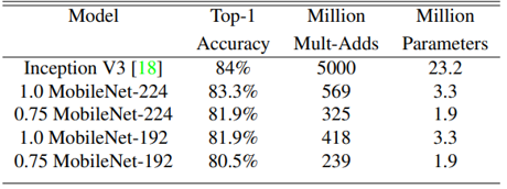
- MobileNet with 𝛼=0.5 and input resolution is 160
- 4% better than AlexNet, while being 45 times smaller and 9.4 times less compute than AlexNet
- 4% better than SqueezeNet, while being same size and 22 times less computation than SqueezeNet
(Table 6. (a) MobileNet comparison to popular model (b) Smaller MobileNet comparison to popular models)
Fine grained recognition
- Training MobileNet with Standford Dogs dataset for classification images of 120 breeds of dogs
- Pretraining with large and noisy web data
- Fine tune the model on the Standford Dogs dataset
- MobileNet can almost achieve the state-of-the-art result with greatly reduced computation and size
(Table 7. Smaller MobileNet comparison to popular models)
Large scale geolocalization
- Training Planet based on the MobileNet using images – location datasets for localizing a large variety of photos
- MobileNet based Planet delivers slightly decreased performance despite more compact than Inception V3 based original Planet
- Still outperforms Image-to-Global Positioning System(Im2GPS)
- Im2GPS estimates location by comparing its feature with a database of geo-tagged photos
(Table 8. Performance of Planet using the Mobilenet)

(Table 9. Comparison of Planets by based model)
Face attributes classification by distillation
- MobileNet can compress large systems with esoteric training procedures
- Synergistic relationship between MobileNet and distillation
- Distill a baseline face attribute classifier using MobileNet architecture
- Training MobileNet to emulate the output of a baseline large model
- Trained on a multi-attribute dataset
- MobileNet based classifier is resilient to aggressive model shrinking
- Achieves a similar mean Average Precision across attribute(mean AP) while consuming only 1 percent the multi-adds
(Table 10. Face attribute classification Using the distillation to MobileNet architecture)
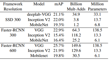
Object detection
- MobileNet is trained on Common Objects in Context(COCO) datasets
- For identifying and locating objects within an image
- MobileNet under both Faster-Regions with CNN(R-CNN) and Single Shot Multibox Detector(SSD)
- SSD is evaluated with 300 input resolution
- Faster R-CNN is evaluated with 300 and 600 input solution
- MobileNet achieves comparable results to other networks with only a fraction of computational complexity and model size
(Table 11. COCO object detection results)
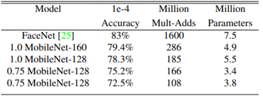
Face embeddings
- The FaceNet model is a state-of-the-art face embedding models
- Embedding face image into 128 dimensions
- Distill a FaceNet model using MobileNet architecture
- Evaluation by face verification task
- Determining whether two peoples in the two photos are the same, whether the distance between two embedded vectors exceed 1e−4
- MobileNet achieves comparable results to other networks with only a fraction of computational complexity and model size
(Table 12. MobileNet distilled from FaceNet)
Conclusion
- Proposed a new model architecture called MobileNets based on depthwise separable convolutions
- Investigated some of the import design decisions
- Demonstrated how to build smaller and faster MobileNets using width multiplier and resolution multiplier
- Compared different MobileNet to popular model, demonstrating superior size, speed and accuracy characteristic
- Concluded by demonstrating effectiveness of MobileNet when applied to a wide variety of tasks
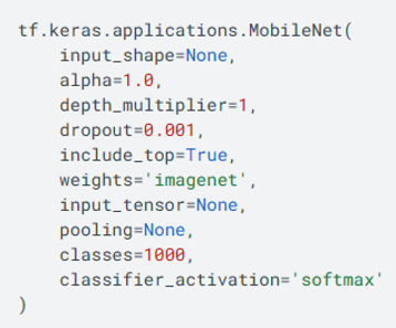
- Plan on releasing models in Tensorflow
- Alpha for width multiplier
- Depth_multiplier for resolution multiplier

(Figure 12. MobileNet on Tensorflow)
Appendix
Running MobileNets with Tensorflow
- You can run Mobilenet pretrained wiht Imagenet on Tensorflow
- Some parameters
- Alpha for width multiplier
- Depth_multiplier for resolution multiplier
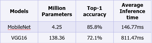
- Less inference time and higher accuracy than VGG16
tf.keras.applications.MobileNet docs
(Figure 21. MobileNet on Tensorflow)
(Table 13. Inference results of pre-trained MobileNet and VGG16 on 1,000 ImageNet images using a CPU(Intel Xeon 2.20GHz) on Colab.)
you can download the Colab code on the link below
Click this link to view the code
Standard convolution layer
- Takes as input a $M\times D_F\times D_F$ feature map $F$, M is number of input channel, $D_F$ is width and height of input feature map
-
Produces a $N\times D_G\times D_G $ feature map $G$, N is number of channel and $D_G$ is width and height of output feature map
- Convolution kernel K of size $M\times N\times D_K\times D_K$
- $M\times D_K\times D_K$ kernel maps $M\times D_K\times D_K$ input into $1\times 1\times 1$
- $M\times N\times D_K\times D_K$ kernel maps $M\times D_K\times D_K$ input into $N\times 1\times 1$
(Figure 14. Standard convolution filters)
Computational cost of standard convolution layer
- assuming one stride and same padding, input spatial size and output spatial size are same
cost of standard convolution layer is \(D_K \times D_K \times M\times N\times D_F \times D_F\)
with number of input channel $M$, number of output channel $N$, Kernel size $D_K\times D_K$, and feature map spatial size $D_F\times D_F$
Each convolution costs $M\times D_K\times D_K$ multiplication, and this convolution applied to each position in the $D_F\times D_F$
Repeat N times to produce N channel output
CNN
- Convolution extracts features using filters that slide over the input
- Padding adds extra pixel around the input to preserve spatial dimensions
- Stride defines the step size of the filter movement, affecting output size
- Pooling reduce spatial dimensions
- Max pooling takes the maximum value from each region
- Average pooling computes the average value from each region
CNN with multiple channels and multiple filters
- Each filter has the same depth as the input channels
- Produce single feature map by combining all channel information
- Multiple filters create multiple feature maps
- Each filter create specific features
RMSProp
- One of the gradient descent optimization algorithm in neural networks
- Gradually decreasing the learning rate as learning progresses
- Gives less weight to gradients from the past
- Gives more weights to recent gradients
Batch normalization
- Normalizes the output of layer using mean and variance of mini-batch
- 𝛾 and 𝛽 are trained by backpropagation
- Normalized with 𝑁(𝛽,𝛾)
Faster R-CNN
RPN
- Feature maps are mapped into low dimension feature map
- With 256x3x3 filters
- Slides over convolutional feature map
- Generates anchor boxes at each position with multiple scales and ratios
- Predicts objectness scores and box coordinates
Fast R-CNN
- Multi class classification and bounding box refinement using top-N RPN
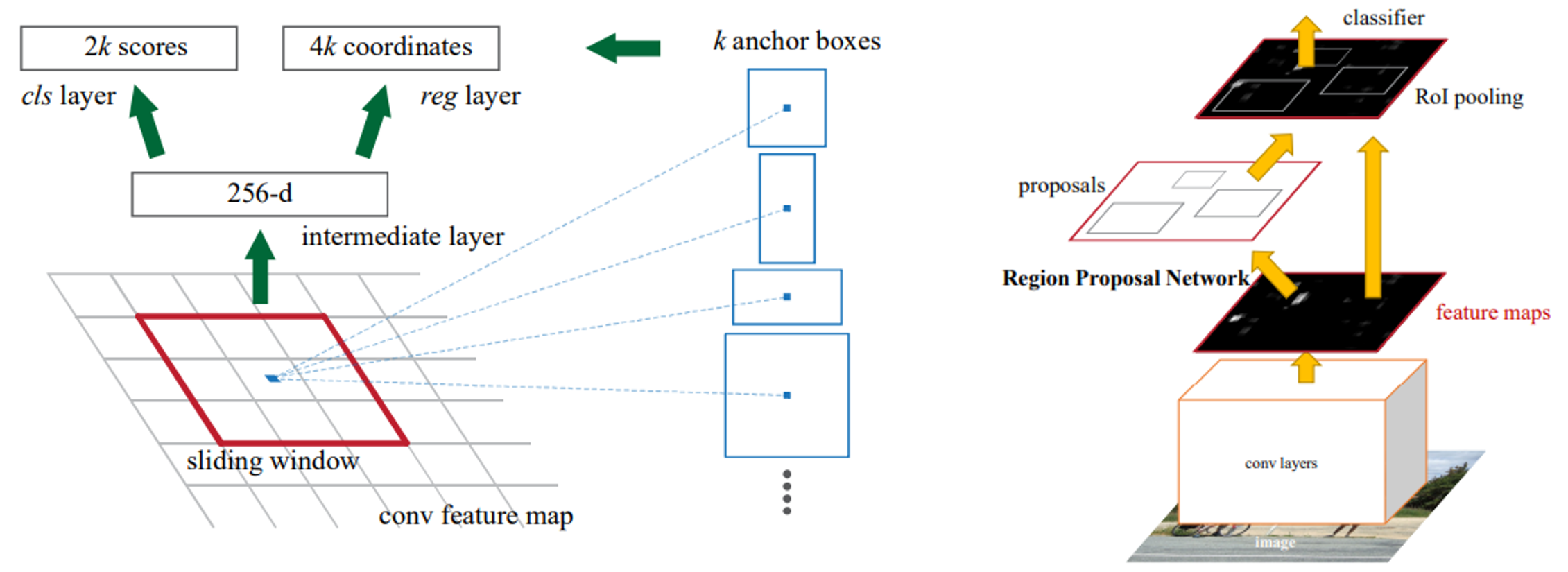
(Figure 15. RPN(left) and Faster R-CNN(right))
SSD
- Employs multi scale feature maps for detecting objects of different sizes
- Extra convolution layers predict bounding boxes and class score
- With 3×3 filter with 𝑘(4+𝑐) channels
- A cell of feature map produce 𝑘 default boxes
- Predict 4 offset and 𝑐 class score per cell of each feature map
- With 3×3 filter with 𝑘(4+𝑐) channels
- Default box has different sizes and ratios
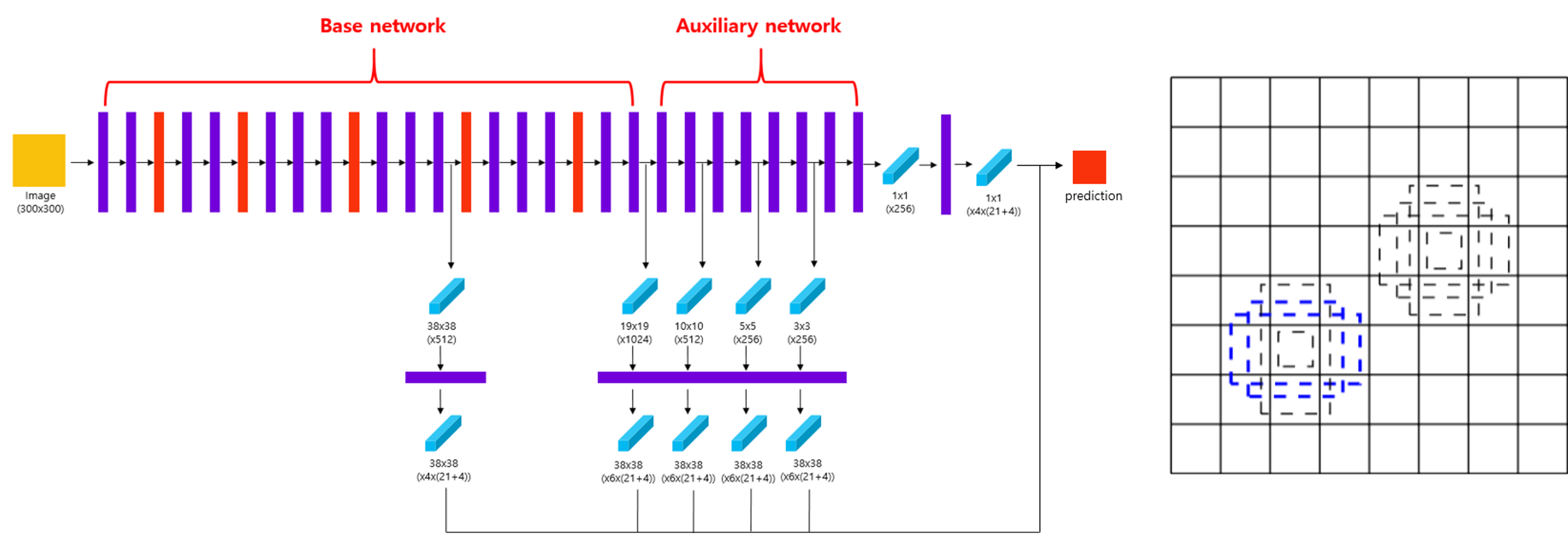
(Figure 16. SSD structure (left) and Default boxes (right))
댓글남기기